Research on Beat Analysis Principles Based on Tempogram

A Study Report on Müller's "Fundamentals of Music Processing" - Chapter 6

Music is not merely a combination of pitch and timbre; it is fundamentally an art of time. When we listen to music, our toes tap instinctively to the beat. This seemingly intuitive human response represents an extremely complex signal processing challenge for computers. My study of this chapter has led me into a crucial domain of Music Information Retrieval (MIR): Tempo and Beat Tracking.

This report systematically presents the complete pipeline from raw audio to discrete beat extraction. It focuses particularly on the core concept of Tempogram, analyzing how it reveals the local tempo characteristics of music.

1. Fundamentals: Onset Detection

The starting point of all rhythm analysis is the occurrence of "events". In signal processing, this is termed Onset Detection.

This task confronts a fundamental challenge: not all instruments exhibit sharp percussive onsets like the piano. For instruments with gradual attacks such as violin or flute, relying solely on energy-based variations often proves inadequate.

A key concept here is spectral-based novelty. By applying Short-Time Fourier Transform (STFT) to the signal and computing spectral differences between adjacent frames (Spectral Flux), we can capture abrupt changes in the frequency distribution of energy. Even when overall energy variation is minimal, changes in spectral content can reveal the onset of new notes. Additionally, this chapter introduces methods utilizing phase instabilities (phase-based) and complex-domain analysis, which further enhance the robustness of onset detection in polyphonic music.

The resulting Novelty Function serves as the fundamental "raw material" for all subsequent rhythm analysis.

2. Core Exploration: Tempogram

If a spectrogram displays "what frequencies occur at what time", then a Tempogram reveals "what tempo dominates at what time." This is the most fascinating part of the chapter.

A tempogram is a three-dimensional representation consisting of a time axis, tempo axis (BPM), and intensity. It not only indicates the overall tempo of a piece but also captures subtle temporal variations in tempo, such as ritardando or accelerando. This chapter provides a detailed comparison of the two primary methods for constructing tempograms. They function as two sides of the same coin:

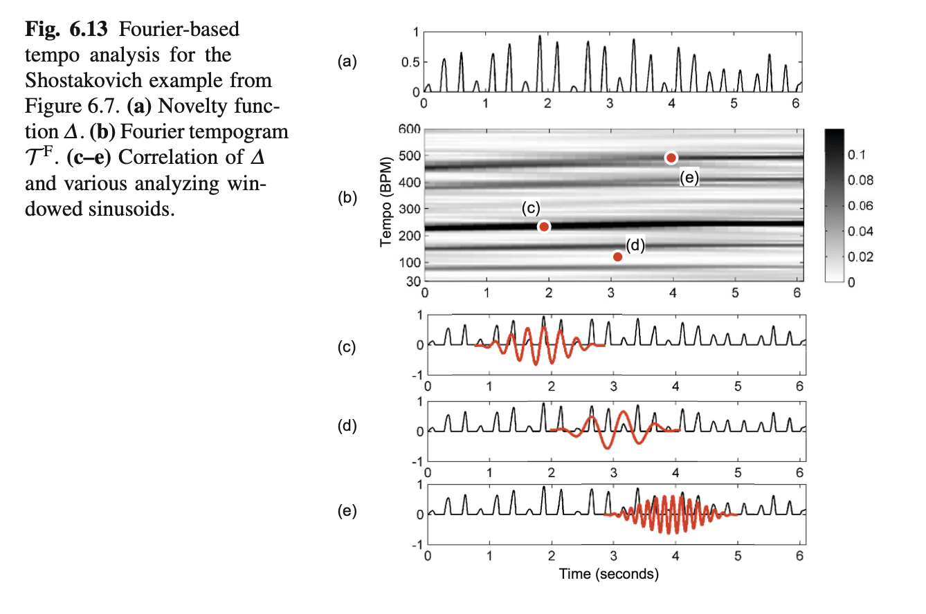
2.1 Fourier Tempogram

This method directly applies short-time Fourier analysis to the Novelty Function.

• Principle: It treats the novelty curve as a time-varying signal and analyzes its frequency components. For instance, a peak occurring every 0.5 seconds corresponds to a frequency of 2 Hz, equivalent to 120 BPM.
• Characteristics: Fourier analysis tends to emphasize tempo harmonics. If a piece has a tempo of 120 BPM, the Fourier tempogram typically exhibits strong energy at 240 BPM and 360 BPM. This occurs because a signal with periodicity at 120 BPM mathematically also satisfies the periodicity at 240 BPM.
• Advantage: It excels at capturing faster pulse levels, such as the tatum level.
  
  

2.2 Autocorrelation Tempogram

This method operates by computing the similarity between the novelty curve and itself at various time lags.

• Principle: If a signal exhibits high self-similarity after a lag of $L$ seconds, then $L$ represents a period.
• Characteristics: In contrast to the Fourier method, autocorrelation tends to emphasize tempo subharmonics. If the fundamental tempo is 120 BPM, the autocorrelation tempogram typically shows peaks at 60 BPM and 30 BPM. This is because if a signal repeats every 0.5 seconds, it naturally also repeats every 1.0 second.
• Advantage: It is more effective at capturing slower pulse levels, such as the measure level.
  
  

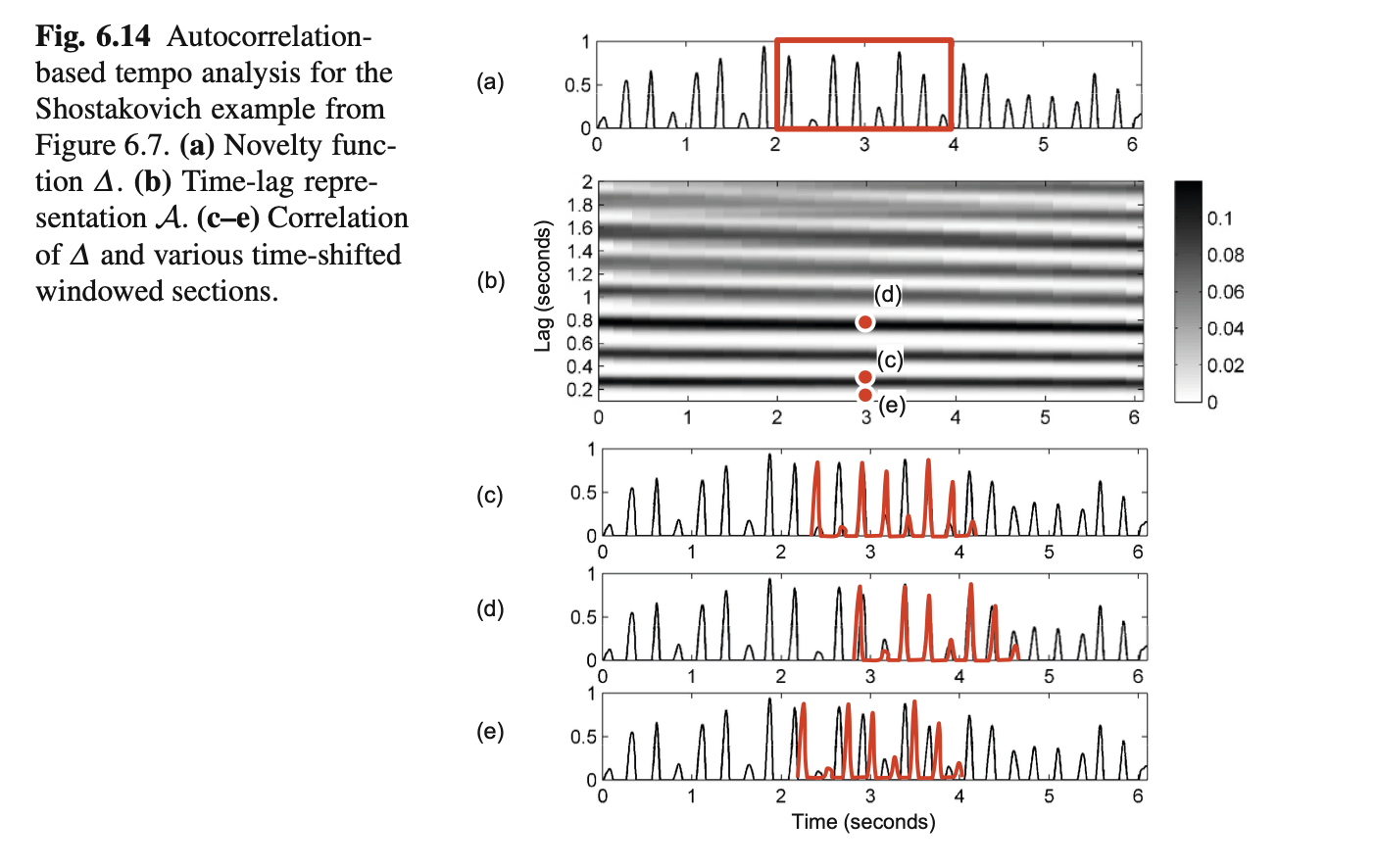
Learning Insight: This chapter brilliantly demonstrates the complementary nature of these two methods through the example of Shostakovich's waltz (Figures 6.13 & 6.14). The waltz is in 3/4 time. The Fourier tempogram clearly reveals the fast rhythm at the quarter-note level, while the autocorrelation tempogram uncovers the slower rhythm at the measure level. In practice, combining both methods often yields more accurate global tempo estimation.

2.3 Cyclic Tempogram

This represents a theoretical elevation in the chapter. Analogous to the chromagram in pitch processing, which groups pitches across octaves into pitch classes, the cyclic tempogram introduces the concept of tempo octaves.

• Definition: Tempi differing by a factor of two (e.g., 60 BPM, 120 BPM, 240 BPM) are treated as equivalent and mapped to the same "cyclic tempo" range.
• Significance: This representation exhibits strong robustness against double-tempo or half-tempo errors. In music structure segmentation, even when different sections are identified at double or half tempo, they still exhibit high homogeneity in the cyclic tempogram. This makes it a powerful mid-level representation.

3. From Tempo to Beat: Tracking and Extraction

With a tempogram, we know "what the tempo is," but we still do not know "where the beat positions are." This is the task of Beat Tracking.

This chapter introduces two strategies:

1. Predominant Local Pulse (PLP): This is an overlap-add-based strategy. It utilizes peak information from the tempogram to construct and superimpose local sinusoids, forming a smooth curve with enhanced periodicity. It essentially "refines" the noisy novelty curve, making the underlying pulse clearly visible.
2. Dynamic Programming (DP): For music with relatively stable tempo, we can define an objective function that both rewards points falling on novelty peaks and penalizes intervals deviating from the expected tempo. Through dynamic programming to find the optimal path, we obtain a globally optimal beat sequence.

4. Conclusion

Chapter 6 not only presents algorithms but also demonstrates a profound understanding of music's essence. From physical-level energy transitions to signal-level periodicity analysis, and finally to musical-level rhythmic hierarchies (tactus, measure, tatum), each transformation aims to approximate human perception of music. The section on tempogram particularly deepened my understanding that "tempo" is not a single number but rather a multi-layered, temporally evolving energy distribution. Whether it is the harmonic characteristics of the Fourier method, the subharmonic characteristics of the autocorrelation method, or the octave invariance of the cyclic tempogram, these all represent sophisticated mathematical lenses we construct in our attempt to teach computers to "comprehend" rhythm.

Appendix (Common Formulas)

STFT and Spectral Representation

• STFT (frame index $n$, frequency bin $k$):

$$
X(n,k)=\sum_{m=0}^{N-1} x[m+nH]\,w[m]\,e^{-j2\pi \frac{k}{N} m}
$$

• Magnitude spectrum:

$$
S(n,k)=|X(n,k)|
$$

• Energy envelope (frame energy, applicable for energy-based onset detection):

$$
E(n)=\sum_{m=0}^{N-1} \bigl(x[m+nH]\,w[m]\bigr)^2
$$

• Frame index to time (seconds):

$$
t(n)=\frac{nH}{f_s}
$$

where $fs$ is the audio sampling rate (Hz). If the novelty frame rate is $f{nov}$, then $t(n)=n / f_{nov}$.

Onset Detection — Energy and Spectral Difference Methods

• Spectral flux (half-wave rectification commonly used):

$$
SF(n)=\sum{k} \bigl[\,S(n,k)-S(n-1,k)\,\bigr]{+}
$$

• Optional normalization (by total energy or local maximum):

$$
\widetilde{SF}(n)=\frac{SF(n)}{\sum_k S(n,k)+\epsilon}
$$

(where $\epsilon$ is a small constant to prevent division by zero)

Phase-based Onset Detection

• Let phase $\phi(n,k)=\arg X(n,k)$, with expected phase advance $2\pi \frac{k}{N}H$. Phase deviation:

$$
\Delta\phi(n,k)=\phi(n,k)-\phi(n-1,k)-2\pi\frac{k}{N}H
$$

• Wrap the deviation to $(-\pi,\pi]$:

$$
\widetilde{\Delta\phi}(n,k)=\mathrm{wrap}\bigl(\Delta\phi(n,k)\bigr)
$$

• Phase-driven novelty (a commonly used form):

$$
PD(n)=\sum_k \bigl|\widetilde{\Delta\phi}(n,k)\bigr|
$$

(or with magnitude weighting: $PD(n)=\sum_k S(n,k)\,|\widetilde{\Delta\phi}(n,k)|$)

Complex-domain Spectral Difference (commonly used to improve performance in polyphonic scenarios)

• Construct predicted values (predicted complex spectrum) using previous frame magnitude and expected phase advance:

$$
\widehat{X}(n,k)=|X(n-1,k)|\,e^{j(\phi(n-1,k)+2\pi\frac{k}{N}H)}
$$

• Complex-domain difference (a commonly used metric):

$$
CD(n)=\sum_k \bigl|X(n,k)-\widehat{X}(n,k)\bigr|
$$

• Or in magnitude/real-part half-wave rectified form:

$$
CD_{+}(n)=\sumk \bigl[\,|X(n,k)|-\Re{\widehat{X}(n,k)}\,\bigr]{+}
$$

(Different literature presents slight variations of complex-domain metrics; the above form is a common interpretable expression)

Novelty Function

• Common construction (based on spectral flux or complex-domain difference):

$$
\nu_{SF}(n)=SF(n)=\sumk [S(n,k)-S(n-1,k)]{+}
$$

or

$$
\nu_{CD}(n)=CD(n)=\sum_k |X(n,k)-\widehat{X}(n,k)|
$$

• The function $\nu(n)$ can be smoothed, normalized, or DC-removed before being used for subsequent rhythm analysis.

Fourier Tempogram

• Apply short-time Fourier transform (or local Fourier transform) to the novelty within a local window to obtain an energy representation in terms of "frequency (Hz)". Let the local window length be $2M+1$ frames with window function $h[m]$:

$$
T{F}(t,f)=\left|\sum{m=-M}^{M} h[m]\,\nu(t+m)\,e^{-j2\pi \frac{f}{f_{nov}} m}\right|
$$

• Map frequency $f$(Hz) to BPM:

$$
\mathrm{BPM}=60\cdot f
$$

• Common discretization: discretize $f$ into the desired BPM grid (e.g., frequencies corresponding to 30–240 BPM).

Autocorrelation Tempogram

• Local (window-weighted) autocorrelation (with frame lag $L$ ):

$$
A(t,L)=\sum_{m=-M}^{M} h[m]\,\nu(t+m)\,\nu(t+m-L)
$$

• Normalized autocorrelation (for comparison):

$$
\widetilde{A}(t,L)=\frac{A(t,L)}{A(t,0)+\epsilon}
$$

• Convert lag $L$(frames) to BPM: if the novelty frame rate is $f_{nov}$(frames/second), then the tempo corresponding to the lag is

$$
\mathrm{BPM}(L)=60\cdot\frac{f_{nov}}{L}
$$

(Note:$L$ is in frames,$L\ge 1$;$L$ corresponds to period $T=L/f_{nov}$ seconds)

Cyclic Tempogram

• Fold tempi according to tempo-octaves (factor-of-two relationships) into the logarithmic periodic domain. Let the reference tempo be $B_{ref}$(e.g., 60 BPM), and the logarithmic position of a tempo $B$ is:

$$
\theta(B)=\log2!\bigl(\tfrac{B}{B{ref}}\bigr)
$$

• Take the fractional part (period of 1, merging each tempo octave):

$$
\theta_c(B)=\theta(B)-\lfloor \theta(B)\rfloor \in [0,1)
$$

• The cyclic spectrum can be obtained by summing energy across octaves (integer offsets $o$):

$$
C(t,\thetac)=\sum{o\in\mathbb{Z}} TF\bigl(t,\,B{ref}\cdot 2^{\theta_c+o}/60\bigr)
$$

(In the above formula, $T_F(t,\cdot)$ takes frequency as the argument; in discrete implementations, sum over several $o$ values within the tempo range)

An equivalent approach: periodically fold $T_F(t,B)$ on the logarithmic tempo axis and sum/average to obtain a cyclic tempogram of length 1.

Predominant Local Pulse (PLP) — Common Frequency-domain Reconstruction Approximation

• A common engineering representation: reconstruct the local pulse (local pulse function $p(t)$):

$$
p(t)\approx \sum_{f} T_F(t,f)\,\cos!\bigl(2\pi f t\bigr)
$$

or using discrete frame indices (with reference to frame rate $f_{nov}$):

$$
p(n)\approx \sum_{f} TF(n,f)\,\cos!\bigl(2\pi \tfrac{f}{f{nov}} n \bigr)
$$

• This formula yields an "enhanced periodic curve" suitable for peak-picking to obtain candidate beat positions. Different implementations apply frequency band selection, harmonic weighting, or phase consistency processing to $T_F$ to enhance results.

(Note: Specific implementation details of PLP vary in the literature; the above presents a common and interpretable frequency-to-time-domain reconstruction formula.)

Dynamic Programming-based Beat Tracking (DP Beat Tracking) — General Mathematical Framework

• Objective: Find a beat sequence ${b_1,b_2,\dots,b_M}$(frame indices or time points) on the candidate frame set to maximize the score:

$$
\mathcal{S}({bi})=\sum{i=1}^{M} s(bi) + \sum{i=2}^{M} \log P\bigl(\Delta_i\bigr)
$$

where $s(b)$ is the "score/novelty/intensity" at time $b$ (e.g., interpolated value of $\nu(b)$), $\Delta_i=bi-b{i-1}$ is the adjacent beat interval (in frames or seconds), and $P(\Delta)$ is a probability model for beat intervals (favoring an expected beat interval).

• If $P(\Delta)$ is modeled as Gaussian (or approximately log-Gaussian):

$$
\log P(\Delta)\propto -\frac{(\Delta-\mu)^2}{2\sigma^2}
$$

then maximization is equivalent to minimization:

$$
\sum_{i=1}^{M}-s(bi) + \lambda \sum{i=2}^{M} (\Delta_i-\mu)^2
$$

(where $\lambda$ is related to $\sigma$ and probability model constants). Dynamic programming efficiently finds the optimal sequence on discrete frames.

• Practical DP implementations commonly include:

  • Initial tempo/interval constraint assumptions;

  • Tolerance for double-tempo/half-tempo (allowing $\Delta$ to vary among several tempo-multiple candidates);

  • Boundary conditions and cost normalization.